|

  
|
||
|
|
||
In Chapter 10 Immiscible Displacement of Dake's "Fundamentals of Reservoir Engineering", he provides the following example.
General Input Data
Oil Density, gm/cc |
0.81 |
Water Density, gm/cc |
1.04 |
Oil viscosity [cP] |
5 |
Water viscosity [cP] |
0.5 |
Initial Oil FVF, Boi [rb/stb] |
1.3 |
Current Oil FVF, Bo [rb/stb] |
1.3 |
Water FVF, Bw [rb/stb] |
1 |
Endpoint kro [fraction] |
0.8 |
Endpoint krw [fraction] |
0.3 |
Swc [fraction] |
0.2 |
Sor [fraction] |
0.2 |
Corey Oil Exponent |
3 |
Corey Water Exponent |
2 |
Porosity [fraction] |
0.18 |
Permeability [mD] |
2000 |
Reservoir Thickness [ft] |
40 |
Reservoir Length [ft] |
2000 |
Reservoir Width [ft] |
625 |
Reservoir Dip [degrees] |
0 |
Injection Rate [mstb/d] |
1000 |
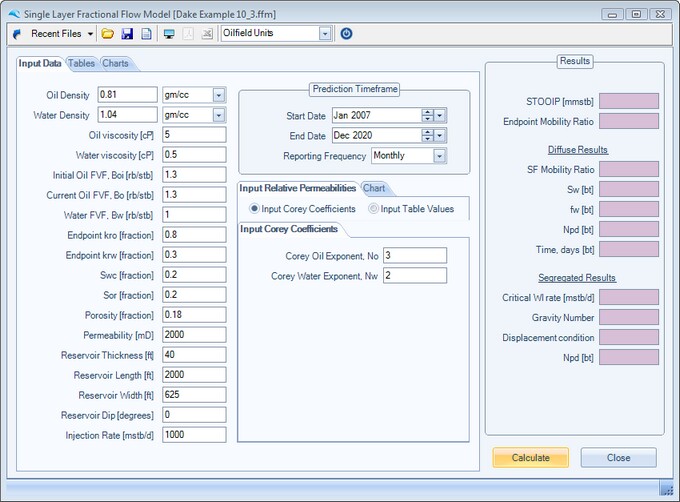
With regards to inputting relative permeability data, the user can choose between using Corey Exponents for Oil and Water curvature or inputting the table values directly. The example below assumes Corey Exponents are input.
Once the user has successfully input all the required data, as shown in the following screen capture, they can press the calculate button to calculate all stages of the performance prediction.
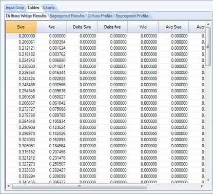
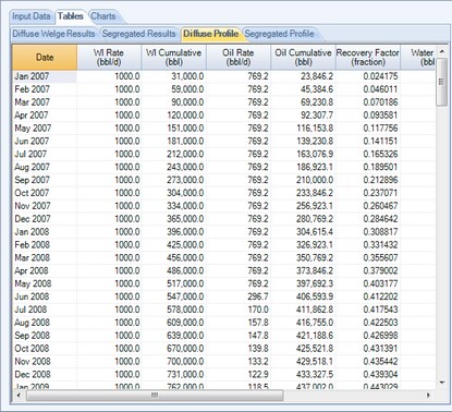
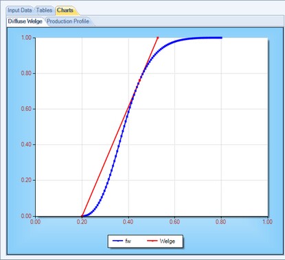
Diffuse Flow Results
The diffuse flow condition results are in the form of tables of Welge calculations and production profile, together with charts of Welge fractional flow and production profiles comparing both the diffuse and segregated flow conditions.
Note that all data within the tables can be output to the clipboard by pressing CTRL+C
|
|
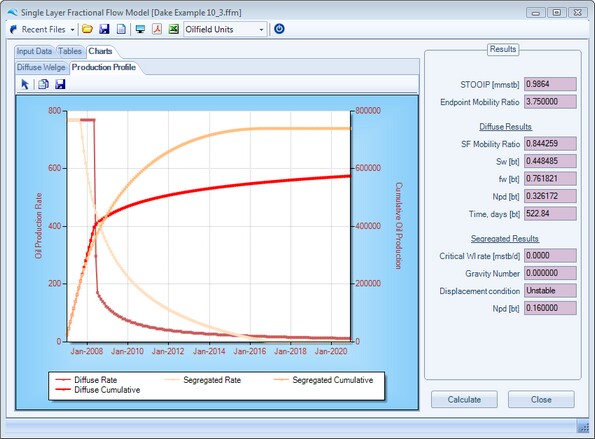
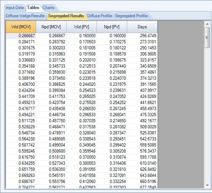
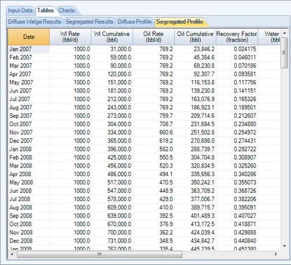
Segregated Flow Results
The segregated flow condition results are in the form of tables of Dake calculations and production profile, together with a production profile chart comparing both the diffuse and segregated flow conditions.
Note that all data within the tables can be output to the clipboard by pressing CTRL+C
|
|
Page url: http://www.YOURSERVER.com/help/index.html?example4.htm