|

  
|
||
|
|
||
Dake provides an example (Example 5.23) in his waterdrive chapter of "The Practice of Reservoir Engineering", which will be used, albeit somewhat modified, to outline this routine in more detail.
Input Data
STOOIP [mmstb] |
126 |
Initial Oil FVF, Boi [rb/stb] |
1.29 |
Current Oil FVF, Bo [rb/stb] |
1.29 |
Water FVF, Bw [rb/stb] |
1 |
Swc, fraction |
0.26 |
Sor, fraction |
0.32 |
Year |
Np |
Wi |
fws |
|
[mmstb] |
[mmstb] |
|
1 |
3.4 |
4.9 |
0.128 |
2 |
11 |
18.9 |
0.356 |
3 |
16.9 |
36.6 |
0.631 |
4 |
21.4 |
55.7 |
0.747 |
5 |
24.9 |
73.7 |
0.794 |
6 |
28 |
92.6 |
0.828 |
7 |
30.5 |
111 |
0.859 |
8 |
32.8 |
130.3 |
0.876 |
9 |
34.8 |
149.2 |
0.891 |
10 |
36.6 |
168.5 |
0.904 |
11 |
38.1 |
187.5 |
0.919 |
12 |
39.5 |
206.9 |
0.926 |
13 |
40.7 |
224.3 |
0.93 |
14 |
41.8 |
242.2 |
0.938 |
15 |
42.7 |
257.9 |
0.942 |
16 |
43.6 |
274 |
0.943 |
17 |
44.4 |
290.1 |
0.949 |
18 |
45.2 |
305.4 |
0.947 |
19 |
45.9 |
321.1 |
0.955 |
20 |
46.6 |
337.6 |
0.957 |
Problem Statement
For the above production history, calculate :
| 1. | the incremental oil production rate in year 21 assuming the water injection system is upgraded from is it's current level of 45,000 bwpd to 80,000 bwpd, |
| 2. | the remaining oil production to an abandonment watercut of 99.9% |
| 3. | The number of years required to reach the abandonment watercut of 99% for both the 45,000 bwpd to 80,000 bwpd levels. |
In this example, the yearly production data has been spline curve fitted to allow the data to be input as monthly data, and formatted into the correct input units. See input screen below.
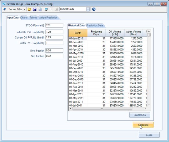
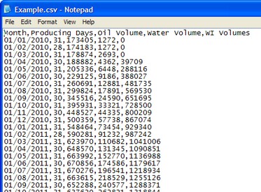
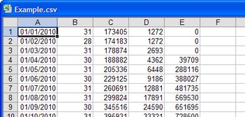
Note that the monthly production and injection history, as per the format shown above, can be input either by importing via a comma delimited ASCII file and by pressing the Import CSV button, or be copied and pasted into the input table by pressing the windows standard shortcut keys [CTRL+C] then [CTRL+V].
Example formats of comma delimited ASCII file (CSV) file are shown below.
|
|
Once the user is happy with the input data they should press the Calculate button, and the following charts and tables should be displayed.
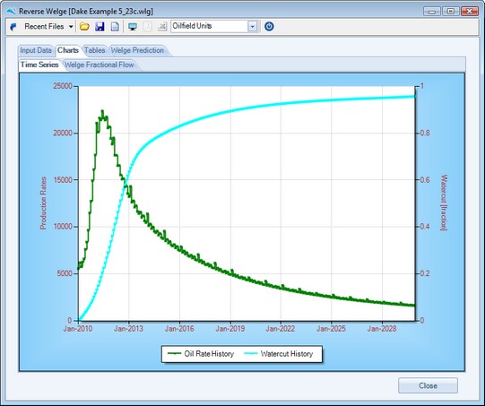
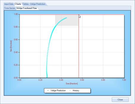
The following chart is the production and injection history data converted to a Welge fractional flow.
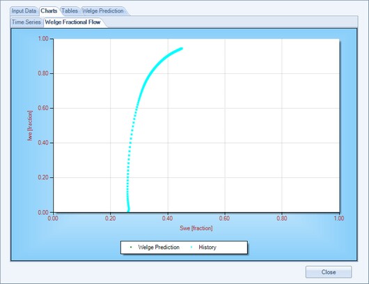
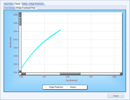
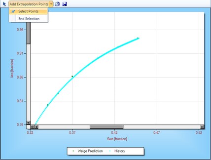
The user can zoom into the late time data to better digitize extrapolation points. To zoom click and drag the left mouse button for the required zoom area. To unzoom press the small icons located in the top of the y-axis scrollbar or at the left edge of the x-axis scrollbar.
|
|
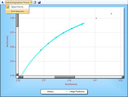
To select extrapolation to digitize, highlight the chart's context menu list by pressing the right mouse button whilst anywhere within the chart area. Then select the "Add Extrapolation Points" & "Select Points", as shown below. Then simply left mouse click where you want to add digitized points. Once the user is happy with the number and location of digitized points, select an area within the margins of the chart (ie,. not in the data display area), and again pressing the right mouse button, select "Add Extrapolation Points" & "End Selection", as shown below.
|
|
The following should be displayed. Although some automatic re-zooming may take place, which may require manually unzooming and re-zooming into the area of interest with the chart.
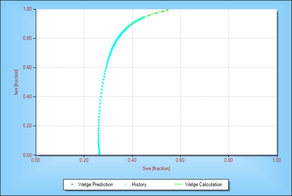
Once the user is happy with the fractional flow extrapolation that have been digitized and curve fitted, they should select the "Welge Prediction" TAB, as shown below.
Within this TAB the user can input a prediction timeframe, facilities constraints and a bestfit prediction function.
The Bestfit Prediction Function returns the coefficients (C1, C2 and C3) of the following equation :
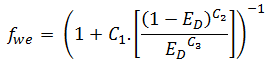
where Ed is the microscopic displacement efficiency, given by the following formula :
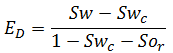
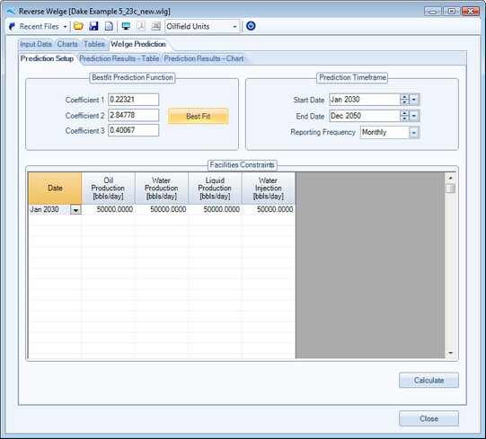
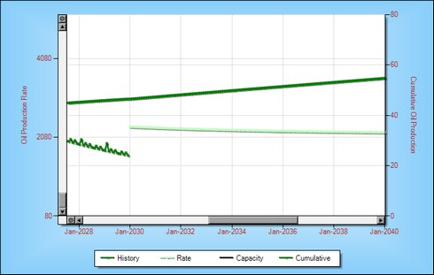
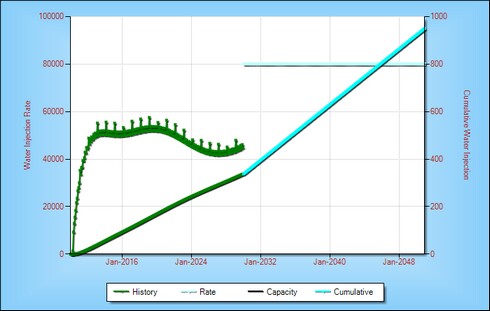
Once the user presses the Calculate button, as shown above, the Welge prediction is performed, for the selected timeframe, using the curve fitted fractional flow extrapolation and the facilities constraints. In this example, for the 45,000 bwpd injection case, the following two screen captures show the predicted water injection and oil production profiles.
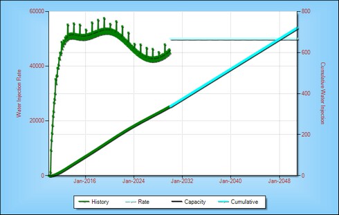
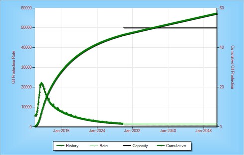
From the above, the prediction is constrained throughout the prediction period by water injection, and the oil production profile appears to merge with history and extrapolate well.
The calculated initial oil rate in year 21 is approximately 2200 bopd, and the ultimate recovery predicted at abandonment watercut is 50.5 mmstb. A remaining reserve figure of 3.9 mmstb,
To quantify the incremental oil production rate for upgrading the water injection capacity to 80,000 bwpd is shown in the following screen captures. The user simplys input the 80,000 bpd for water injection (and water and liquid production, since this will be the next constraint to be met in the prediction calculations) and again presses the Calculate button.
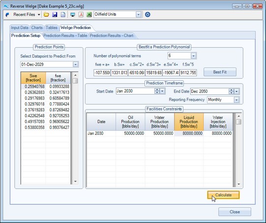
The results for the 80,000 bwpd case are shown below. From these calculations, the oil rate predicted initially in year 21 is approximately 2300 bopd, an incremental oil rate of 600 bopd over the 45,000 bwpd injection case. The 80,000 bwpd injection case also reaches 50.5 mmstb ultimate recovery, but 5 years earlier.
Obviously the additional capital expenditure required to upgrade injection capacity may be more than offset by the acceleration of oil production and the saving of 5 years field operating expenditure.
Page url: http://www.YOURSERVER.com/help/index.html?example5.htm