|

  
|
||
|
|
||
In Chapter 5 Waterdrive of Dake's "The Practice of Reservoir Engineering", he provides the following example.
General Input Data
Oil Density, gm/cc |
0.7 |
Water Density, gm/cc |
1.02 |
Oil Viscosity [cP] |
1.24 |
Water Viscosity [cP] |
0.41 |
Oil FVF, Bo rb/stb |
1.475 |
Water FVF, Bw rb/stb |
1.03 |
Water FVF, Bw rb/stb |
1.03 |
Reservoir Length [ft] |
4000 |
Reservoir Width [ft] |
1000 |
Reservoir Dip, degrees |
10 |
Injection Rate [stb/d] |
6000 |
Selected Method |
Stiles |
STOOIP [mmstb] |
176 |
Use Areal Sweep Correlation ? |
True |
Select Pattern Method |
Direct Line Drive |
Layer Input Data
Layer |
Thickness |
Porosity |
Permeability |
Swc |
Sor |
kro |
krw |
|
[ft] |
[fraction] |
[mD] |
[fraction] |
[fraction] |
[fraction] |
[fraction] |
|
|
|
|
|
|
|
|
1 |
8 |
0.259 |
2840 |
0.168 |
0.33 |
1 |
0.33 |
2 |
9 |
0.25 |
2000 |
0.165 |
0.33 |
1 |
0.33 |
3 |
13 |
0.253 |
1560 |
0.175 |
0.33 |
1 |
0.33 |
4 |
4 |
0.22 |
74 |
0.192 |
0.33 |
1 |
0.33 |
5 |
8 |
0.235 |
1244 |
0.18 |
0.33 |
1 |
0.33 |
6 |
6 |
0.228 |
718 |
0.187 |
0.33 |
1 |
0.33 |
7 |
11 |
0.227 |
650 |
0.195 |
0.33 |
1 |
0.33 |
8 |
14 |
0.215 |
32 |
0.205 |
0.33 |
1 |
0.33 |
9 |
14 |
0.22 |
320 |
0.196 |
0.33 |
1 |
0.33 |
10 |
7 |
0.213 |
34 |
0.21 |
0.33 |
1 |
0.33 |
Problem Statement
For the above data, calculate :
| 1. | the reservoir fractional flow and resultant oil recovery versus watercut relationships assuming a Stiles, no vertical pressure communication between layers, method, |
| 2. | the likely field STOOIP value, given a knowledge of the production history. |
| 3. | the future oil, water, liquid production and water injection profiles assuming the following facilities constraints; 60mbbl/d oil, 60mbbl/d water and 65mbbl/d liquid production and 65mbbl/d water injection. |
Once the user has input all the necessary input data, they should press the Calculate button, as shown below. Note that the layer data can be copied and pasted into the input table by pressing the windows standard shortcut keys [CTRL+C] then [CTRL+V].

The fractional flow data will be calculated and displayed in the following TAB, as shown below.

Since all the required data has been input to calculate synthetic production log versus various watercut values based on each layer's water breakthrough, we have provided the display and layer calculations for these synthetic production logs. See example provided below.

Once the fractional flow data has been successfully calculated, proceed to the next TAB, Welge Displacement, as shown below, and press the Calculate Welge Displacement button.

The user can choose to bestfit a regression equation to better describe the Npd v's fws relationship, for later use in the prediction calculations, see following screen capture.
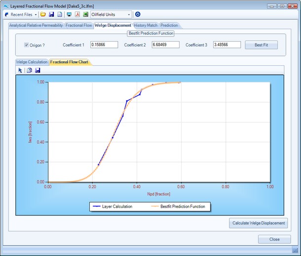
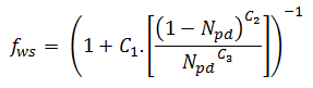
The Bestfit button returns the coefficients (C1, C2 and C3) of the following equation :
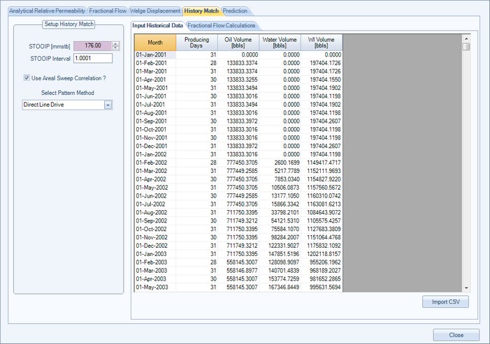
History Matching
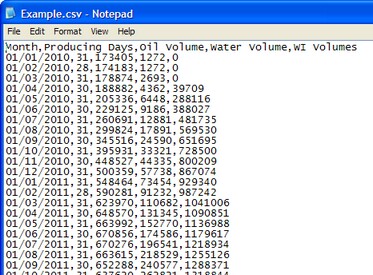
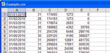
If the oilfield under study is a producing field and the monthly values of production and injection history are known, then the User can choose to history match the total field oil originally in place, STOOIP. This is illustrated in the following screen captures. Firstly enter the monthly production and injection history, as per the format shown below, either by importing via a comma delimited ASCII file and by pressing the Import CSV button, or via copy [CTRL+C] and paste [CTRL+V] from an external application such as Microsoft Excel into the data input table below.
Example formats of comma delimited ASCII file (CSV) file are shown below.
|
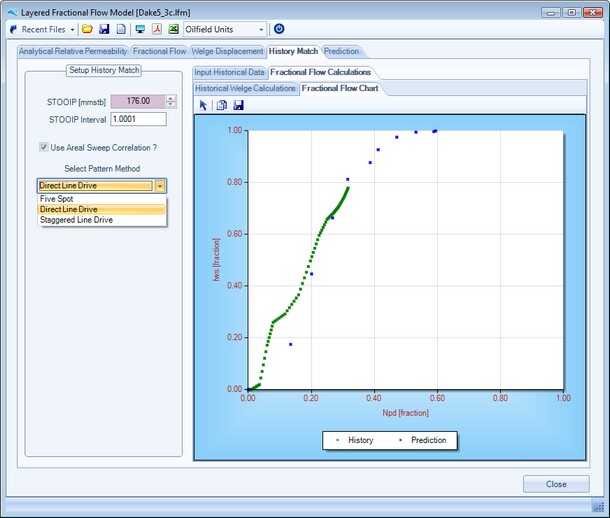
|
The user can then iterate the STOOIP value by selecting the up and down buttons adjacent to the STOOIP value, as shown below, to iterate the fractional flow history match. The user can also choose to modify the vertical layer predicted values of fws v's NpD by applying an areal sweep correlation. To enable this option simply select the Use Areal Sweep Correlation check box and then select the waterdrive pattern; namely 5 spot, direct line drive or staggered line drive.
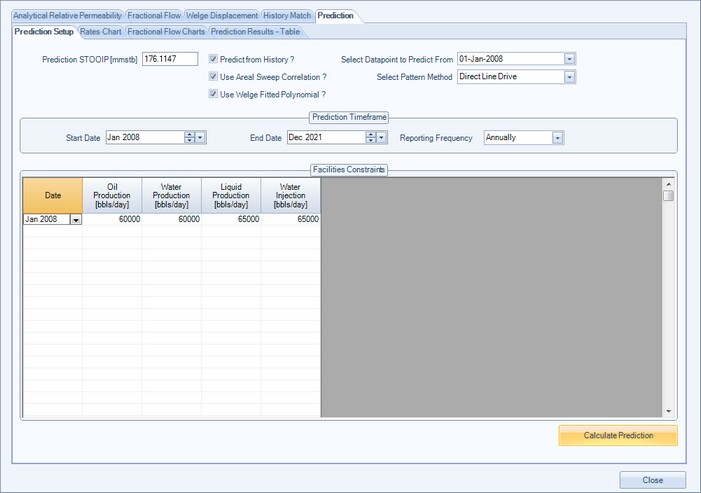
Prediction Performance
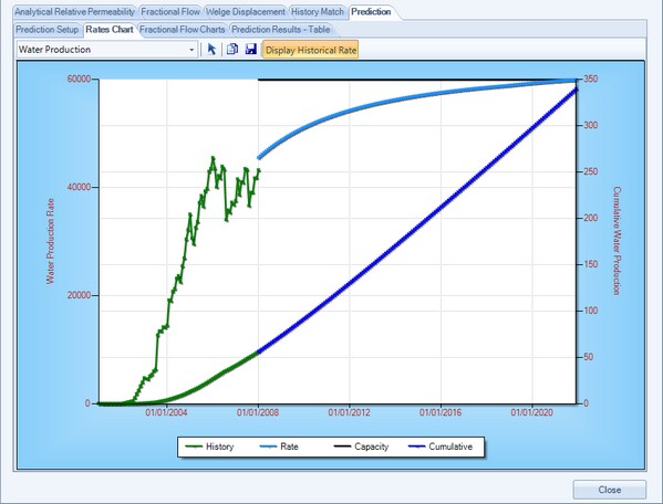
To calculate the prediction performance, select the Prediction tab. Enter appropriate values for STOOIP, check whether to predict values from History, whether to use an areal sweep correlation in the prediction calculations, and whether to use the best fit Welge polynomial calculated in the Welge Displacement tab. Once the prediction timeframe has been entered together with the facilities constraints, the user can press the Calculate Prediction button, as shown below.
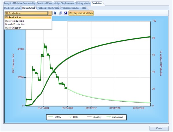
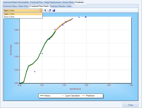
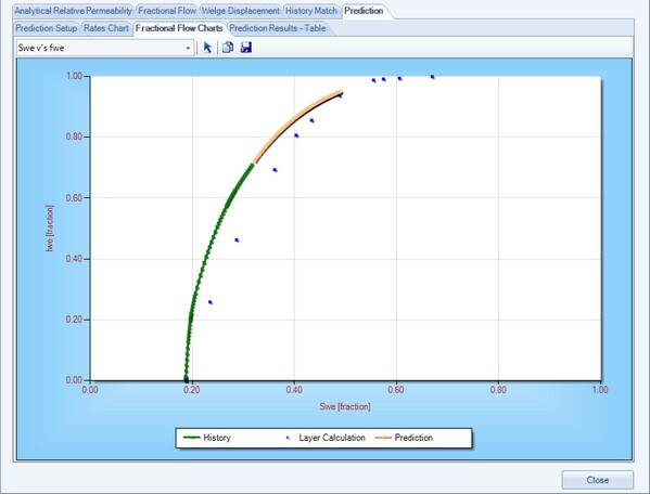
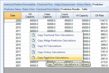
Various charts and tables of prediction output are shown as examples below.
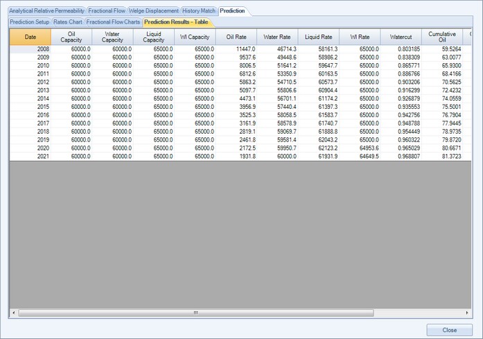
The user can copy any of the data to the Windows clipboard from any of the tables by either, clicking and dragging an area with their mouse and pressing CTRL+C, then pasting into an external application, or when the mouse is over a active table single right click the mouse to display the tables context menu then select the table that requires to be copied. The benefits of selecting the second approach over the first approach is that the table headers will also be be copied to the clipboard. See screen capture below.
References:
Fassihi, M., “New Correlations for Calculation of Vertical Coverage and Areal Sweep Efficiency,” SPERE, Nov. 1986
Page url: http://www.YOURSERVER.com/help/index.html?example7.htm