|

  
|
||
|
|
||
In terms of Waterdrive decline analysis, the Log(Water Oil Ratio) v's Cumulative Oil Production (or Np) to predict oil recoveries for water oil ratios (WOR) greater than 1 or watercut greater than 50% is commonplace.
Therefore we have developed a simple routine to permit low, mid and high trend decline analysis of Log(WOR) v's Np relationships. The user can also convert to an oil production rate v's time series, by either assuming a starting oil rate or by a constant liquid production rate, which for steady state waterdrive fields is also a commonplace assumption.
The following series of screen captures describe how to use this workflow :
The user can copy and paste (via CTRL+C and CTRL+V) production data into the Input Data Table - just select the top left data cell as highlighted below, or choose to import data via the Import CSV button also shown below. The user can also choose to optionally input the Stock Tank Oil Originally in Place (STOOIP) and the application will automatically calculate recovery efficiencies versus time.
The historical data frequency used can be defined by the User, but we advise to input monthly production figures, as all of the prediction calculations are done with a monthly prediction frequency.
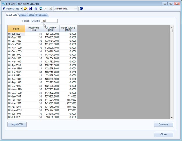
Once the production data has been successfully input, the user should press the Calculate Button, as shown above, to populate the calculation Table and Chart.
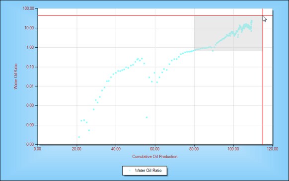
On the Charts Tab the following Log(WOR) v's Cumulative Oil Production chart is displayed. The user can choose to zoom into the display to better digitize points for curve fitting a linear relationship. This functionality is shown below and is enabled by left mouse clicking and dragging a highlighted box. Once happy with the selected area, unrelease the mouse button and the chart area will zoom in.
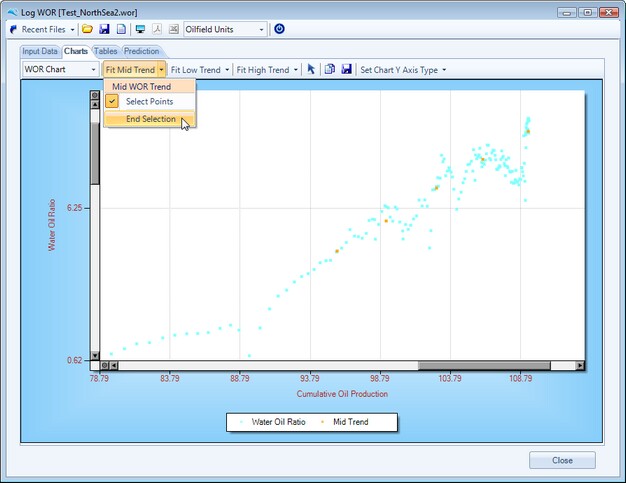
To select points to be fitted, select the Select Points button as shown below for the Fit Mid Trend. The process can be repeated for the Low and High trend analysis.
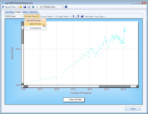
Once the Select Points button has been selected and highlighted, the user can select points directly in the chart area, by a series of single right mouse clicks, as shown below.
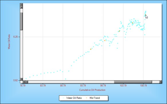
Once all of the required points have been selected, select the End Selection button, to fit a straight line through the selected points, as shown below.
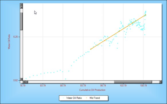
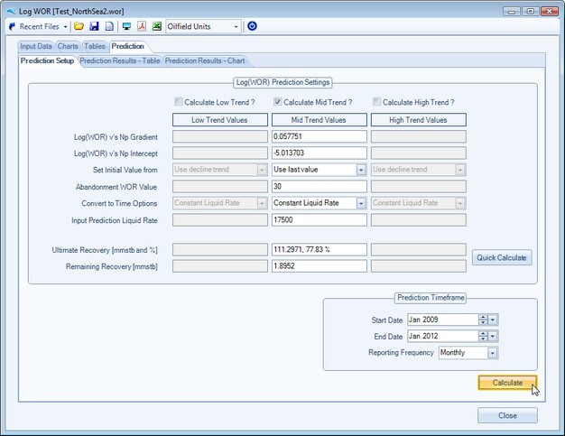
Once a straight line has been fitted through through the selected points, the User can see the Gradient and Intercept values associated with the straight line in the Prediction Tab, as shown below.
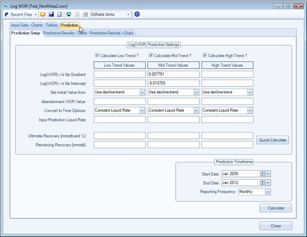
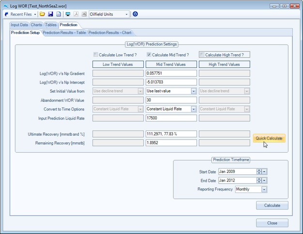
To convert to time or quickly calculate Ultimate and remaining recovery, the user should input Abandonment assumptions for Water Oil ratio and select how to convert to time, as shown below. The Quick Calculate button only uses the fitted linear relationship and intersects this with the Abandonment WOR value.
To convert the prediction to time, the user also needs to enter the start date, end date and reporting frequency. All internal calculations are done monthly, however the user can choose to report either monthly, semi annually or annually. This is shown for illustration purposes below :
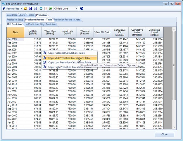
Once the user enters the prediction input correctly and presses the Calculate button, as shown above, the Prediction tables and Charts are populated. The User can copy the Table data from the application by a single right mouse click, to select the table Context menus. as shown below :
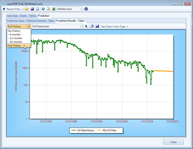
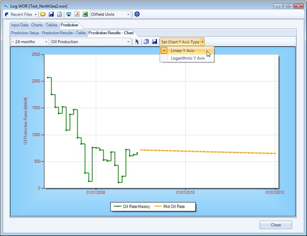
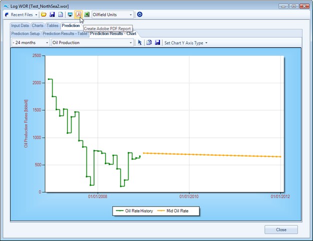
Various display elements of the prediction chart can be changed for both historical production, prediction phase (either Oil, Water or Total Liquids) and Y Axis type, see below :
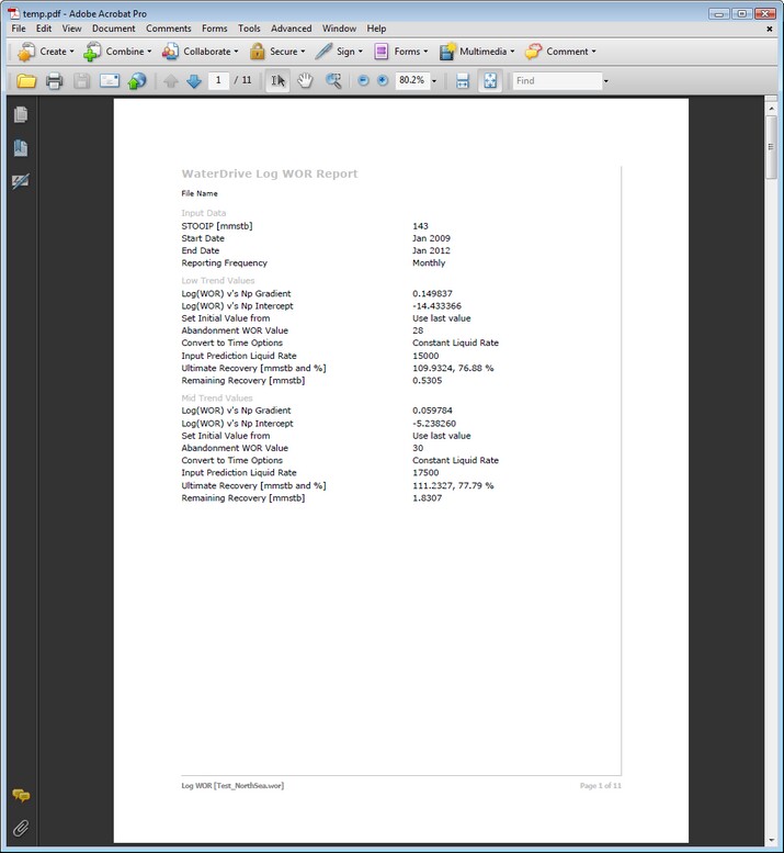
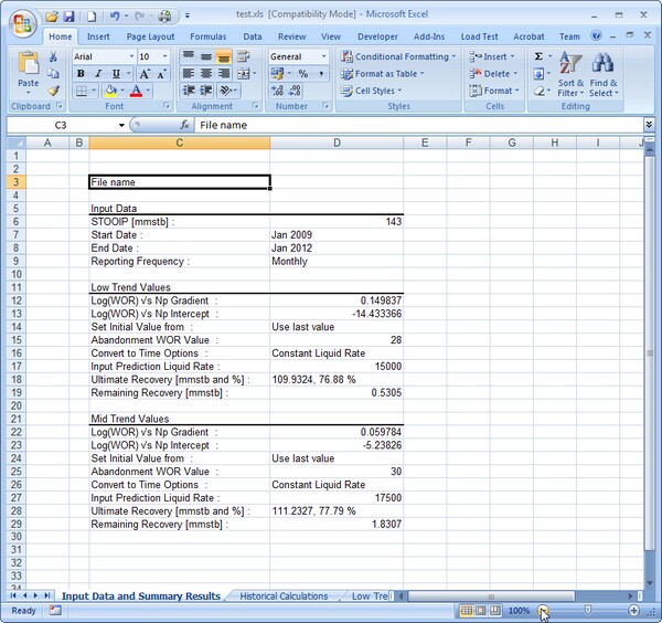
Once happy with the prediction sensitivities, the user can create either Adobe PDF or Microsoft Excel reports, as depicted below :
Page url: http://www.YOURSERVER.com/help/index.html?log_wor_decline_forecasts.htm